As an engineering student, my biggest challenge is the time it takes me to manually solve a system of equations during exams, as these are not the point of interest but rather a necessary step to tackle the real problem.
In my search for a method to speed things up, I found three worth mentioning:
Cramer's rule
This is a theorem from linear algebra that provides the solution to a linear system of equations in terms of determinants. It is named after Gabriel Cramer (1704-1752), who published the rule in his Introduction à l'analyse des lignes courbes algébriques in 1750.
Cramer's Rule is of theoretical importance because it gives an explicit expression for the solution of the system. However, for systems of more than three equations, its application for solving becomes excessively costly. Nonetheless, as it does not require matrix pivoting, it is more efficient than Gaussian elimination for small matrices, particularly when SIMD operations are used.
Knowing this, I can assume it won't be the best method for solving my system, but I will try it anyway to see how it truly develops.
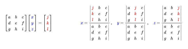
So, if Ax=b is a system of equations, A is the coefficient matrix of the system, x=(x1, …, xn) is the column vector of the unknowns, and b is the column vector of the constants, then the solution to the system is presented as follows:
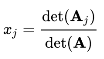
Where Aj is the matrix resulting from replacing the j-th column of A by the column vector b. It should be noted that for the system to be determined compatible, the determinant of matrix A must be non-zero.
To obtain determinants in matrices larger than 3×3, Laplace expansion is used to reduce them, and once a 3×3 system is reached, Sarrus's Rule is applied.
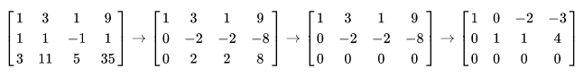
Gaussian method
Named after Carl Friedrich Gauss (1777-1855), this algorithm is used to transform the matrix of a system of linear equations into an upper triangular matrix by reducing the system to an equivalent one where each new equation has one less unknown than the previous one, ultimately leading to the solutions
The method consists of:
1- Starting at the first column, moving from left to right.
2- If the first row has a zero in this column, swap it with another row that does not have a zero.
3- Obtain zeros below this leading element by adding suitable multiples of the top row to the rows below it.
4- Move to the next column in the next row and repeat the previous process with the remaining submatrix.
5- Repeat with the rest of the rows (at this point, the matrix is in echelon form).
Once the echelon form is obtained, it follows that the last value of the augmented part is the result of the last unknown. This value is then used to calculate the other unknowns upwards.
Vega method
I have not been able to find official information about this method, so I do not know its true name or original author; therefore, it should be used at discretion. In my opinion, I can say that the method has worked well for me in the years I have been applying it.
This method was published on July 23, 2016, on YouTube by Mechatronics Engineer Héctor Manuel Vega, a professor at San Buenaventura University, Colombia. video on YouTube
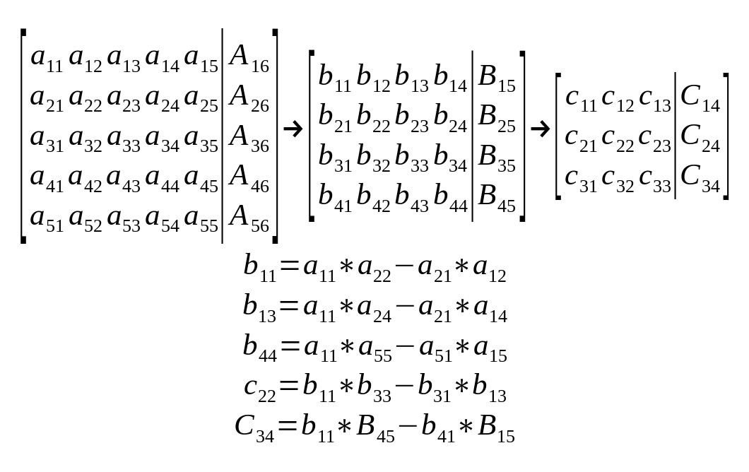
The method consists, like Gauss's, of a reduction of the original matrix but using determinant calculations. The calculation process takes the first value of the matrix (a₁₁) as the pivot, which will be multiplied by a value that remains within the imaginary reduced matrix (without row a₁j and column aᵢ₁). This value is then subtracted from the product of a₁j and aᵢ₁, where i and j correspond to the selected value within the imaginary matrix. This result will be called bij. By repeating this procedure for all values of the imaginary matrix, an equivalent matrix of one degree less will be formed. This reduction must be repeated as many times as there are unknowns. In the end, we will obtain a simple equation from which the last variable is isolated, allowing us to determine the others by going back through the already calculated reduced matrices.
The idea now is to compare the steps needed to solve the system of equations with each of the methods, also considering the traditional method. For this, I will use a system of six equations with six unknowns, as it is a fairly common system in my daily life.
Matrix to use as an example:
Resolution
8*x1+0*x2+1*x3+5*x4+3*x5+8*x6=1
1*x1+9*x2+1*x3+4*x4+7*x5+4*x6=6
7*x1+4*x2+1*x3+3*x4+2*x5+6*x6=8
5*x1+5*x2+1*x3+0*x4+9*x5+7*x6=4
0*x1+0*x2+3*x3+9*x4+6*x5+8*x6=2
6*x1+4*x2+0*x3+3*x4+5*x5+7*x6=9
8*x1+x3+5*x4+3*x5+8*x6=1
x1=1/8-1/8*x3-5/8*x4-3/8*x5-x6
x1+9*x2+x3+4*x4+7*x5+4*x6=6
1/8-1/8*x3-5/8*x4-3/8*x5-x6+9*x2+x3+4*x4+7*x5+4*x6=6
x2=47/72-7/72*x3-3/8*x4-53/72*x5-1/3*x6
7*x1+4*x2+x3+3*x4+2*x5+6*x6=8
7*(1/8-1/8*x3-5/8*x4-3/8*x5-x6)+4*(47/72-7/72*x3-3/8*x4-53/72*x5-1/3*x6)+x3+3*x4+2*x5+6*x6=8
x3=-325/19-207/19*x4-257/19*x5-168/19*x6
5*x1+5*x2+x3+9*x5+7*x6=4
5*(1/8-1/8*x3-5/8*x4-3/8*x5-x6)+5*(47/72-7/72*x3-3/8*x4-53/72*x5-1/3*x6)-325/19-207/19*x4-257/19*x5-168/19*x6+9*x5+7*x6=4
5*(1/8-1/8*(-325/19-207/19*x4-257/19*x5-168/19*x6)-5/8*x4-3/8*x5-x6)+5*(47/72-7/72*(-325/19-207/19*x4-257/19*x5-168/19*x6)-3/8*x4-53/72*x5-1/3*x6)-325/19-207/19*x4-257/19*x5-168/19*x6+9*x5+7*x6=4
x4=17/36+47/36*x5+25/72*x6
3*x3+9*x4+6*x5+8*x6=2
3*(-325/19-207/19*x4-257/19*x5-168/19*x6)+9*(17/36+47/36*x5+25/72*x6)+6*x5+8*x6=2
3*(-325/19-207/19*(17/36+47/36*x5+25/72*x6)-257/19*x5-168/19*x6)+9*(17/36+47/36*x5+25/72*x6)+6*x5+8*x6=2
x5=-129/131-107/262*x6
6*x1+4*x2+3*x4+5*x5+7*x6=9
6*(1/8-1/8*x3-5/8*x4-3/8*x5-x6)+4*(47/72-7/72*x3-3/8*x4-53/72*x5-1/3*x6)+3*(17/36+47/36*x5+25/72*x6)+5*(-129/131-107/262*x6)+7*x6=9
6*(1/8-1/8*(-325/19-207/19*x4-257/19*x5-168/19*x6)-5/8*(17/36+47/36*x5+25/72*x6)-3/8*(-129/131-107/262*x6)-x6)+4*(47/72-7/72*(-325/19-207/19*x4-257/19*x5-168/19*x6)-3/8*(17/36+47/36*x5+25/72*x6)-53/72*(-129/131-107/262*x6)-1/3*x6)+3*(17/36+47/36*x5+25/72*x6)+5*(-129/131-107/262*x6)+7*x6=9
6*(1/8-1/8*(-325/19-207/19*(17/36+47/36*x5+25/72*x6)-257/19*(-129/131-107/262*x6)-168/19*x6)-5/8*(17/36+47/36*(-129/131-107/262*x6)+25/72*x6)-3/8*(-129/131-107/262*x6)-x6)+4*(47/72-7/72*(-325/19-207/19*(17/36+47/36*x5+25/72*x6)-257/19*(-129/131-107/262*x6)-168/19*x6)-3/8*(17/36+47/36*(-129/131-107/262*x6)+25/72*x6)-53/72*(-129/131-107/262*x6)-1/3*x6)+3*(17/36+47/36*(-129/131-107/262*x6)+25/72*x6)+5*(-129/131-107/262*x6)+7*x6=9
6*(1/8-1/8*(-325/19-207/19*(17/36+47/36*(-129/131-107/262*x6)+25/72*x6)-257/19*(-129/131-107/262*x6)-168/19*x6)-5/8*(17/36+47/36*(-129/131-107/262*x6)+25/72*x6)-3/8*(-129/131-107/262*x6)-x6)+4*(47/72-7/72*(-325/19-207/19*(17/36+47/36*(-129/131-107/262*x6)+25/72*x6)-257/19*(-129/131-107/262*x6)-168/19*x6)-3/8*(17/36+47/36*(-129/131-107/262*x6)+25/72*x6)-53/72*(-129/131-107/262*x6)-1/3*x6)+3*(17/36+47/36*(-129/131-107/262*x6)+25/72*x6)+5*(-129/131-107/262*x6)+7*x6=9
x6=5,7452
x5=-129/131-107/262*5,7452 --> x5=-3,3311
x4=17/36-47/36*3,3311+25/72*5,7452 --> x4=-1,8819
x3=-325/19+207/19*1,8819+257/19*3,3311-168/19*5,7452 --> x3=-2,3446
x2=47/72+7/72*2,3446+3/8*1,8819+53/72*3,3311-1/3*5,7452 --> x2=2,1234
x1=1/8+1/8*2,3446+5/8*1,8819+3/8*3,3311-5,7452 --> x1=-2,9018
TOTAL TIME: 114 MINUTES
Results obtained by MatLab:
x1 = -2,902
x2 = 2,124
x3 = -2,346
x4 = -1,882
x5 = -3,331
x6 = 5,745
Results of the traditional method and the associated error:
x1 = -2,9018 - e% = 0,007%
x2 = 2,1234 - e% = 0,028%
x3 = -2,3446 - e% = 0,059%
x4 = -1,8819 - e% = 0,005%
x5 = -3,3311 - e% = 0,003%
x6 = 5,7452 - e% = 0,003%
|8 0 1 5 3 8| |1|
|1 9 1 4 7 4| |6|
A=|7 4 1 3 2 6| b=|8|
|5 5 1 0 9 7| |4|
--> |0 0 3 9 6 8| |2|
|6 4 0 3 5 7| |9|
Laplace
|8 0 5 3 8| |8 0 1 3 8| |8 0 1 5 8| |8 0 1 5 3|
|1 9 4 7 4| |1 9 1 7 4| |1 9 1 4 4| |1 9 1 4 7|
det(A)=3*(-1)^(5+3)*|7 4 3 2 6|+9*(-1)^(5+4)*|7 4 1 2 6|+6*(-1)^(5+5)*|7 4 1 3 6|+8*(-1)^(5+6)*|7 4 1 3 2|=
|5 5 0 9 7| |5 5 1 9 7| |5 5 1 0 7| |5 5 1 0 9|
|6 4 3 5 7| |6 4 0 5 7| |6 4 0 3 7| |6 4 0 3 5|
A1 A2 A3 A4
--> |8 0 5 3 8|
|1 9 4 7 4|
A1=|7 4 3 2 6|
|5 5 0 9 7|
|6 4 3 5 7|
Laplace
|9 4 7 4| |1 9 7 4| |1 9 4 4| |1 9 4 7|
det(A1)=8*(-1)^(1+1)*|4 3 2 6|+5*(-1)^(1+3)*|7 4 2 6|+3*(-1)^(1+4)*|7 4 3 6|+8*(-1)^(1+5)*|7 4 3 2|=
|5 0 9 7| |5 5 9 7| |5 5 0 7| |5 5 0 9|
|4 3 5 7| |6 4 5 7| |6 4 3 7| |6 4 3 5|
A11 A12 A13 A14
|9 4 7 4|
A11=|4 3 2 6|
--> |5 0 9 7|
|4 3 5 7|
Laplace
|4 7 4| |9 4 4| |9 4 7|
det(A11)=5*(-1)^(3+1)*|3 2 6|+9*(-1)^(3+3)*|4 3 6|+7*(-1)^(3+4)*|4 3 2|=
|3 5 7| |4 3 7| |4 3 5|
applying Sarrus
det(A11)=5*(-1)^(3+1)*(4*2*7+7*6*3+4*3*5-4*6*5-7*3*7-4*2*3)+9*(-1)^(3+3)*(9*3*7+4*6*4+4*4*3-9*6*3-4*4*7-4*3*4)+7*(-1)^(3+4)*(9*3*5+4*2*4+7*4*3-9*2*3-4*4*5-7*3*4)=
det(A11)=-377
TIME TO THIS POINT: 52 MINUTES
ESTIMATED TIME TO OBTAIN THE FIRST DETERMINANT: 298 MINUTES
TOTAL ESTIMATED TIME (seven necessary determinants): 2086 MINUTES (approximately 30 hours)
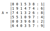
|8 0 1 5 3 8 : 1|
|1 9 1 4 7 4 : 6|
|7 4 1 3 2 6 : 8|
|5 5 1 0 9 7 : 4|
|0 0 3 9 6 8 : 2|
|6 4 0 3 5 7 : 9|
|1,000 0,000 0,125 0,625 0,375 1,000 : 0,125|
|0,000 9,000 0,875 3,375 6,625 3,000 : 5,875|
|0,000 4,000 0,125 -1,375 -0,625 -1,000 : 7,125|
|0,000 5,000 0,375 -3,125 7,125 2,000 : 3,375|
|0,000 0,000 3,000 9,000 6,000 8,000 : 2,000|
|0,000 4,000 -0,750 -0,750 2,750 1,000 : 8,250|
|1,000 0,000 0,125 0,625 0,375 1,000 : 0,125|
|0,000 1,000 0,097 0,375 0,736 0,333 : 0,653|
|0,000 0,000 -0,263 -2,875 -3,569 -2,332 : 4,513|
|0,000 0,000 -0,110 -5,000 3,445 0,335 : 0,110|
|0,000 0,000 3,000 9,000 6,000 8,000 : 2,000|
|0,000 0,000 -1,138 -2,250 -0,194 -0,332 : 5,638|
|1,000 0,000 0,125 0,625 0,375 1,000 : 0,125|
|0,000 1,000 0,097 0,375 0,736 0,333 : 0,653|
|0,000 0,000 1,000 10,932 13,570 8,867 : -17,160|
|0,000 0,000 0,000 -3,797 4,938 1,310 : -1,778|
|0,000 0,000 0,000 -23,796 -34,710 -18,601 : 53,480|
|0,000 0,000 0,000 10,191 15,249 9,759 : -13,890|
|1,000 0,000 0,125 0,625 0,375 1,000 : 0,125|
|0,000 1,000 0,097 0,375 0,736 0,333 : 0,653|
|0,000 0,000 1,000 10,932 13,570 8,867 : -17,160|
|0,000 0,000 0,000 1,000 -1,301 -0,345 : 0,468|
|0,000 0,000 0,000 0,000 -65,669 -26,811 : 64,617|
|0,000 0,000 0,000 0,000 28,507 13,275 : -18,659|
|1,000 0,000 0,125 0,625 0,375 1,000 : 0,125|
|0,000 1,000 0,097 0,375 0,736 0,333 : 0,653|
|0,000 0,000 1,000 10,932 13,570 8,867 : -17,160|
|0,000 0,000 0,000 1,000 -1,301 -0,345 : 0,468|
|0,000 0,000 0,000 0,000 1,000 0,408 : -0,984|
|0,000 0,000 0,000 0,000 0,000 1,644 : 9,392|
|1,000 0,000 0,125 0,625 0,375 1,000 : 0,125|
|0,000 1,000 0,097 0,375 0,736 0,333 : 0,653|
|0,000 0,000 1,000 10,932 13,570 8,867 : -17,160|
|0,000 0,000 0,000 1,000 -1,301 -0,345 : 0,468|
|0,000 0,000 0,000 0,000 1,000 0,408 : -0,984|
|0,000 0,000 0,000 0,000 0,000 1,000 : 5,713|
x6 = 5,713
x5 = -0,984-0,408x6 --> x5 = -3,315
x4 = 0,468+0,345*x6+1,301*x5 --> x4 = -1,874
x3 = -17,160-8,867*x6-13,570*x5-10,932*x4 --> X3 = -2,346
x2 = 0,653-0,333*x6-0,736*x5-0,375*x4-0,097*x3 --> x2 = 2,121
x1 = 0,125-x6-0,375*x5-0,625*x4-0,125*x3 --> x1 = -2,880
TOTAL TIME: 72 MINUTES
Results obtained by MatLab:
x1 = -2,902
x2 = 2,124
x3 = -2,346
x4 = -1,882
x5 = -3,331
x6 = 5,745
Results of the Gauss method and the associated error:
x1 = -2,9018 - e% = 0,758%
x2 = 2,1234 - e% = 0,141%
x3 = -2,3446 - e% = 0,000%
x4 = -1,8819 - e% = 0,425%
x5 = -3,3311 - e% = 0,480%
x6 = 5,7452 - e% = 0,557%
|8 0 1 5 3 8 : 1|
|1 9 1 4 7 4 : 6|
|7 4 1 3 2 6 : 8|
|5 5 1 0 9 7 : 4|
|0 0 3 9 6 8 : 2|
|6 4 0 3 5 7 : 9|
|72 7 27 53 24 : 47|
|32 1 -11 -5 -8 : 57|
|40 3 -25 57 16 : 27|
| 0 24 72 48 64 : 16|
|32 -6 -6 22 8 : 66|
|-152 -1656 -2056 -1344 : 2600|
| -64 -2880 1984 192 : 64|
|1728 5184 3456 4608 : 1152|
|-656 -1296 -112 -192 : 3248|
| 331776 -433152 -115200 : 156672|
|2073600 3027456 1622016 : -4667904|
|-889344 -1331712 -852480 : 1211904|
| 1,9026e12 7,7702e11 : -1,8736e12|
|-8,2705e11 -3,8528e11 : 5,4142e11|
|-9,0399e22 : -5,1926e23|
x6=-5,1926e23/-9,0399e22 --> x6 = 5,744
x5=(-1,8736e12-7,7702e11*x6)/1,9026e12 --> x5 = -3,331
x4=(156672+115200*x6+433152*x5)/331776 --> x4 = -1,882
x3=(2600+1344*x6+2056*x5+1656*x4)/(-152) --> x3 = -2,334
x2=(47-24*x6-53*x5-27*x4-7*x3)/72 --> x2 = 2,123
x1=(1-8*x6-3*x5-5*x4-x3)/8 --> x1 = -2,902
TOTAL TIME: 48 MINUTES
Results obtained by MatLab:
x1 = -2,902
x2 = 2,124
x3 = -2,346
x4 = -1,882
x5 = -3,331
x6 = 5,745
Results of the Vega method and the associated error:
x1 = -2,9018 - e% = 0,000%
x2 = 2,1234 - e% = 0,047%
x3 = -2,3446 - e% = 0,512%
x4 = -1,8819 - e% = 0,000%
x5 = -3,3311 - e% = 0,000%
x6 = 5,7452 - e% = 0,017%
----------------------------------------------------
By being able to solve systems of equations of up to 3 unknowns with my calculator, I can simplify calculations, saving time and reducing errors.
|8 0 1 5 3 8 : 1|
|1 9 1 4 7 4 : 6|
|7 4 1 3 2 6 : 8|
|5 5 1 0 9 7 : 4|
|0 0 3 9 6 8 : 2|
|6 4 0 3 5 7 : 9|
|72 7 27 53 24 : 47|
|32 1 -11 -5 -8 : 57|
|40 3 -25 57 16 : 27|
| 0 24 72 48 64 : 16|
|32 -6 -6 22 8 : 66|
|-152 -1656 -2056 -1344 : 2600|
| -64 -2880 1984 192 : 64|
|1728 5184 3456 4608 : 1152|
|-656 -1296 -112 -192 : 3248|
| 331776 -433152 -115200 : 156672|
|2073600 3027456 1622016 : -4667904|
|-889344 -1331712 -852480 : 1211904|
solve system of equations with calculator:
x4 = -1,882
x5 = -3,331
x6 = 5,745
I resume manual calculations
x3=(2600+1344*x6+2056*x5+1656*x4)/(-152) --> x3 = -2,343
x2=(47-24*x6-53*x5-27*x4-7*x3)/72 --> x2 = 2,123
x1=(1-8*x6-3*x5-5*x4-1*x3)/8 --> x1 = -2,902
TOTAL TIME: 39 MINUTES
Results obtained by MatLab:
x1 = -2,902
x2 = 2,124
x3 = -2,346
x4 = -1,882
x5 = -3,331
x6 = 5,745
Results of the Vega method + calculator, and the associated error:
x1 = -2,9018 - e% = 0,000%
x2 = 2,1234 - e% = 0,047%
x3 = -2,3446 - e% = 0,128%
x4 = -1,8819 - e% = 0,000%
x5 = -3,3311 - e% = 0,000%
x6 = 5,7452 - e% = 0,000%
Once the resolutions are completed, I obtain the following data:
-Traditional method: 114 minutes
-Cramer's rule: 2086 minutes (estimated value from partial resolution)
-Gauss method: 72 minutes
-Vega method: 48 minutes
Having the results, I was very surprised to see how slow Cramer’s Rule becomes for matrices larger than 3×3; it was much more than I expected, which led me to abandon the resolution when I was approximately 1/6 through the resolution of the first determinant after 52 minutes, with 7 determinants to resolve.
In case you are interested in how I obtained the estimated time, it was as follows:
22min(Laplace 5x5)+17min(Laplace 4x4)*6+13min(Laplace 3x3 + Sarrus)*24 = 436min/det
436min/det * 7det = 3052 minutes → about 51 hours
This is what it would take me to fully solve a 6×6 matrix using this method. It is worth noting that in my example, I took advantage of the existence of empty values to reduce the time to 298 minutes per determinant, resulting in the total time of 2086 minutes described above.
Traditionally, it was as expected; I solved the exercise in 114 minutes. It was a long and tedious process, where one must be careful not to confuse any values or signs.
With the Gaussian method, a lot of time is saved; it is straightforward to follow without getting lost and does not generate much error (around 0.4%).
Lastly, the Vega method. By far my favorite on the list, it is very quick to resolve, simple to carry out, and introduces almost no error (just under 0.1%). Additionally, during the process, it generates equivalent matrices of one degree less per step, allowing the resolution of equations with a simple scientific calculator upon reaching a 3×3 matrix, thus improving the time to 39 minutes and reducing the error to 0.03%.
If you wish to see and review the step-by-step resolutions, they are available at the following link. Along with these, there is also a small program in C that applies the Vega method to matrices of up to 10×10, showing the step-by-step process until reaching the final result.